The difference between the Probability Density Function (PDF) and the Cumulative Distribution Function (CDF) in Layman’s terms…

The Probability Density Function (PDF) of a variable indicates how likely it is to find the variable at a specific value. For a standard normal distribution with mean 0 and standard deviation 1, the PDF is expressed as:

φ(x) = 1 / (√(2 * π)) * e^(-x^2 / 2)

The value of φ(x) at any point x gives the relative likelihood of the variable occurring near that point. To find the probability that the variable lies between two points, you calculate the area under the curve of φ(x) from one point to the other.

The Cumulative Distribution Function (CDF) provides the probability that the variable will be less than or equal to a value x. For the standard normal distribution, the CDF at point x is calculated by integrating the PDF from negative infinity up to x:

N(x) = ∫ from -∞ to x of φ(t) dt

The CDF increases from 0 to 1 as x moves from left to right across the number line. At x=0, the midpoint of the bell curve, N(0) is 0.5, indicating there's a 50% chance the variable will be less than or equal to zero, due to the symmetry of the curve.

In simpler language:

• φ(x) tells us the density of probability at a particular point x.
• N(x) tells us the probability of the variable being less than or equal to x.

Making the bridge between the CDF and the PDF:

For option pricing, the CDF values N(d1) and N(d2) are critical for the Black-Scholes model, which helps determine the theoretical price of options.

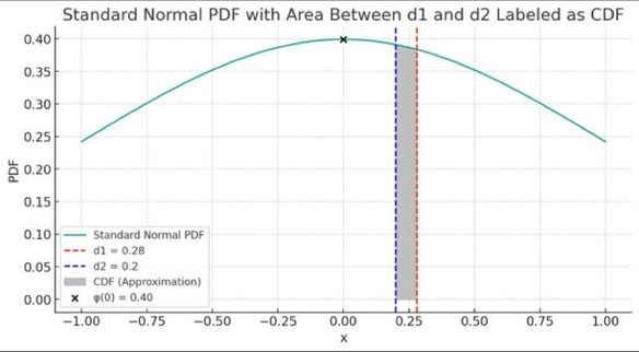
When we approximate the difference between N(d1) and N(d2) for values of d1 and d2 that are close to each other, we can use the fact that the PDF φ(x) is almost constant between d1 and d2 if they are near the center of the distribution (x = 0). So, we can approximate the difference in the CDFs, N(d1) - N(d2), as the area under the PDF curve between d1 and d2:

N(d1) - N(d2) ≈ φ(0) * (d1 - d2) (*)

Substituting the value for φ(0), we get:

N(d1) - N(d2) ≈ (1 / (√(2 * π))) * (d1 - d2)

1 / (√(2 * π)≈ 0.4

This approximation is a practical way to estimate the probability that a normally distributed random variable falls between d1 and d2, which is a frequent calculation in financial models like the Black-Scholes formula for option pricing.


(*)

Area of a rectangle = height * width.

hashtag#ProbabilityDensityFunction hashtag#CumulativeDistributionFunction hashtag#StandardNormalDistribution hashtag#OptionPricing hashtag#BlackScholesModel hashtag#StatisticalApproximation hashtag#FinancialMathematics hashtag#RiskAssessment hashtag#QuantitativeAnalysis