The SABR (Stochastic-Alpha-Beta-Rho) model in layman’s terms…

The SABR (Stochastic Alpha Beta Rho) model is a stochastic volatility model. It is used in quantitative finance to describe the dynamics of the volatility of an underlying asset, typically in the context of options pricing and risk management.
This model was introduced in 2002 by Patrick Hagan, Deep Kumar, Andrew Lesniewski, and Diana Woodward and has since become a standard tool for practitioners in the financial industry.

The SABR model considers the following key equations:

The asset price (S) follows geometric Brownian motion, similar to the Black-Scholes model:

- dS = μS dt + σS dW₁

Where:
- dS is the infinitesimal change in asset price.
- μ is the drift rate.
- σ is the instantaneous volatility of the asset.
- dt is the infinitesimal time step.
- dW₁ is a Wiener process (Brownian motion) representing randomness.

The volatility (σ) follows a stochastic process:

- dσ = ασ dW₂

Where:
- dσ is the infinitesimal change in volatility.
- α is the parameter representing the volatility of volatility.
- dW₂ is another Wiener process, independent of dW₁.

The SABR model uses three main parameters:

- Alpha (Alpha): Alpha represents the initial volatility level.
- Beta (Beta): Beta is a parameter that determines how the volatility reacts to changes in the asset's price. It's often called the "elasticity" parameter.
- Rho (Rho): Rho represents the correlation between the asset's price movements and the volatility movements. It measures how the two are related.

The SABR model introduces another parameter called "nu" (Nu), which controls the volatility of volatility. This parameter captures how much the asset's volatility itself is expected to change over time.

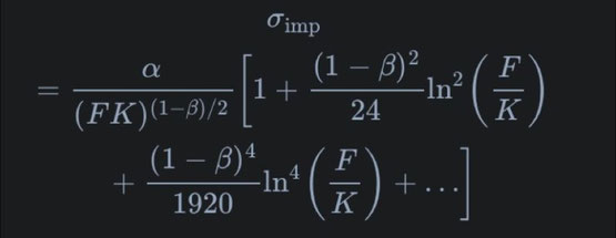
One of the primary uses of the SABR model is to calibrate its parameters to observed market data, such as option prices. This calibration process involves finding the values of alpha, beta, rho, and nu that best fit the observed market prices. The primary use of the SABR model is to calculate the implied volatility (σ_imp) for a given option price.

These equations provide the foundation for the SABR model. However, solving the SABR model analytically for option pricing can be complex due to nonlinearities, so numerical methods or approximation techniques are often used in practice. The SABR model is valued for its ability to capture the dynamics of volatility and is widely used in quantitative finance for pricing and managing options and derivatives.

#SABRModel #QuantitativeFinance #VolatilityModeling#OptionsPricing #StochasticModel #FinancialDerivatives#ImpliedVolatility #AssetPriceDynamics #RiskManagement#OptionTrading #MathFinance #QuantitativeAnalysis#FinancialModels #VolatilitySurface #MarketRisk #DerivativesPricing#AlphaBetaRho #FinancialMath #AssetPricing