The Cheyette model offers a simplified approach to modeling interest rates compared to the Heath-Jarrow-Morton (HJM) model while maintaining enough flexibility to capture complex interest rate structures. Notably, it reduces the dimensionality of the calculations, allowing for faster simulations, making it attractive for many applications. However, this relative simplicity hides a sophistication that makes it more complex to calibrate compared to models like Vasicek or Hull-White.

Dimensionality Simplification

Unlike HJM, where forward interest rate dynamics are modeled in an infinite state space (each maturity being modeled separately), the Cheyette model simplifies this by reducing it to a finite number of state variables. This transition from infinite to finite dimensions significantly speeds up calculations and facilitates numerical simulations, especially in contexts where precision must be balanced with time constraints.

The Markovian Structure: Optimized Predictions

One of the most striking aspects of the Cheyette model is its Markovian structure. Unlike the HJM model, which requires accounting for the entire history of interest rates to predict their future evolution, the Cheyette model relies solely on the current state. This means that forward rates can be modeled as a Markov process with a finite number of state variables, greatly simplifying calculations. This Markovian property stems from the Cheyette model's ability to reduce HJM’s infinite dimensionality to a finite number of state variables while still capturing the essential forward rate dynamics.

Sequential Approximation of Volatilities and the Stone-Weierstrass Theorem

The Cheyette model allows any forward rate dynamics to be approximated by progressively increasing the number of state variables. This sequential approximation approach enables the modeling of complex volatility structures while limiting the model’s dimensionality, adding flexibility while making calculations more manageable.

The Stone-Weierstrass Theorem justifies this approach by proving that any continuous function, such as interest rate volatility, can be approximated by a polynomial with arbitrary precision. In other words, this theorem ensures that the complexity of the HJM model can be captured with more simplicity in the Cheyette model without losing precision in the rate dynamics.

Comparison with Unifactorial Models: More Flexibility but More Complexity

Compared to unifactorial models like Vasicek and Hull-White, the Cheyette model offers greater flexibility, especially with parameters that depend on both time and maturity. While Vasicek is based on mean reversion and constant volatility, and Hull-White allows time variability, the Cheyette model offers more nuanced modeling at the cost of more complex calibration. This increased calibration effort is a natural tradeoff for the added flexibility, making it ideal for modeling complex yield curve dynamics.

Despite its increased flexibility compared to unifactorial models, the Cheyette model remains simpler than HJM for several reasons:

• Dimensionality Reduction: The Cheyette model shifts from an infinite dimension to a finite number of state variables, greatly reducing computational burdens, particularly for simulations.
• Markovian Dependence: Unlike HJM, the Cheyette model does not require retaining the entire history of interest rates. By relying only on the current state, it allows for more efficient and faster modeling without sacrificing precision.

Mathematical Formulation of the Cheyette Model

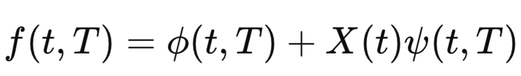
The forward rate dynamics in the Cheyette model are governed by a stochastic differential equation (SDE) of the following form:

\[ df(t, T) = \alpha(t, T) [\theta(t, T) \cdot f(t, T)] \, dt + \sigma(t, T) \, dW(t) \]

where:

• \( t \): Current time.
• \( T \): Maturity of the forward rate.
• \( \alpha(t, T) \): Controls the mean reversion speed of the interest rate and may depend on both time and maturity.
• \( \theta(t, T) \): Average level to which the forward rate reverts.
• \( \sigma(t, T) \): Forward rate volatility, depending on time and maturity.
• \( dW(t) \): Wiener process (Brownian motion).

This equation highlights two key terms:

• \( \alpha(t, T) [\theta(t, T) \cdot f(t, T)] \): Captures mean reversion, forcing the rate back to a predefined average level.
• \( \sigma(t, T) dW(t) \): Represents the random fluctuations due to market uncertainties.

Why is the Cheyette Model Less Popular?

The Cheyette model, while powerful and flexible, is not as well-known or as widely used as the Vasicek, Hull-White, or Cox-Ingersoll-Ross (CIR) models for several reasons:

• The Cheyette model's parameters can depend on both time and maturity, making the model more sophisticated. While this can be a strength, it also means the model requires more extensive data and greater calibration effort. This can be off-putting to practitioners who need a quick and intuitive model.
• Due to its multifaceted nature, the Cheyette model can be computationally more demanding. In real-world applications where speed can be crucial, simpler models like Vasicek or CIR might be preferred.
• Vasicek and CIR models have been around longer and were some of the first to address mean reversion in interest rates. They've had more time to gain acceptance, get implemented in standard software, and be taught in academic courses.
• Models like Vasicek and CIR are relatively straightforward in their mathematical structure, making them easier to teach, learn, and apply. Their simplicity makes them intuitive for many financial practitioners.