The Carr & Madan Approach to Option Pricing, Simply Explained

The Fourier Transform is a powerful mathematical tool that allows a function \( f(x) \) to be expressed as a sum of frequencies. Mathematically, this is written as:

\[ F(v) = \int f(x) e^{-i v x} dx \]

The inverse Fourier Transform allows us to recover the original function:

\[ f(x) = \frac{1}{2\pi} \int F(v) e^{i v x} dv \]

The function \( F(v) \) is a complex number, which consists of two key components: amplitude and phase.

Amplitude: \( A(v) = |F(v)| \) → represents the strength of each frequency component.

Phase: \( \phi(v) = \arg(F(v)) \) → describes the shift in oscillations.

A function that is smooth, such as an option price with a long maturity, is primarily dominated by low-frequency components. This means that high amplitudes occur around \( v \approx 0 \).

In contrast, a sharp function, like an option price with a short maturity, contains more high-frequency components, resulting in high amplitudes for \( v \gg 0 \).

When the option price evolves smoothly with respect to the strike, it is well represented by low frequencies. However, if discontinuities appear, such as intrinsic value effects, the function introduces significant high-frequency components.

Pricing a Call Option

The price of a European call option is given by the following integral:

\[ C_T(k) = e^{-rT} \int_k^\infty (e^s - e^k) q_T(s) ds \]

where \( q_T(s) \) represents the risk-neutral density function.

For large maturities \( T \), the function \( C_T(k) \) remains smooth, and its Fourier Transform is dominated by low-frequency components. However, for small \( T \), the function approaches its intrinsic value, introducing discontinuities.

These discontinuities create a significant presence of high-frequency components, making Fourier inversion unstable. The integral becomes highly oscillatory, complicating numerical computations.

The Carr & Madan Adjustment

Instead of working directly with \( C_T(k) \), Carr & Madan focus on the time value component of the option price, defined as:

\[ z_T(k) = C_T(k) - \max(e^k - S_0, 0) \]

Here, \( \max(e^k - S_0, 0) \) represents the intrinsic value of the option. Unlike \( C_T(k) \), the function \( z_T(k) \) tends to zero at both extremes, mitigating instabilities.

When \( k \ll \ln(S_0) \), meaning the option is deep in-the-money, the intrinsic value dominates. The time value is minimal, leading to \( z_T(k) \to 0 \) as \( k \) decreases.

Conversely, when \( k \gg \ln(S_0) \), meaning the option is deep out-of-the-money, the intrinsic value is zero. In this case, \( C_T(k) = z_T(k) \), and as \( k \) increases, \( C_T(k) \) decays exponentially, causing \( z_T(k) \to 0 \).

While \( C_T(k) \) does not vanish at extremes, leading to instability in Fourier Transform calculations, \( z_T(k) \) naturally vanishes at both ends, avoiding high-frequency distortions. However, for \( k = 0 \) and as \( T \to 0 \), \( z_T(k) \) becomes extremely sharp, resembling a Dirac delta function.

This transformation results in a broadened Fourier Transform, increasing oscillations and numerical instability.

Stabilizing the Fourier Transform

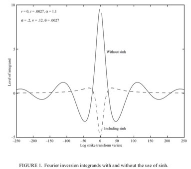
To address this instability, Carr & Madan introduce a modification by multiplying \( z_T(k) \) with \( \sinh(\alpha k) \):

\[ \tilde{z}_T(v) = \int \sinh(\alpha k) \cdot z_T(k) e^{-i v k} dk \]

The function \( \sinh(\alpha k) \) vanishes at \( k = 0 \), effectively eliminating parasitic oscillations. This stabilizes the Fourier Transform and improves numerical accuracy in option pricing computations.

Graph source: Option Valuation Using the Fast Fourier Transform, Carr and Madan