
Maximum likelihood estimation is a statistical technique used to estimate the parameters of a probabilistic model from observed data. It aims to find the parameter values that make the observed data most probable, i.e., those that maximize the probability of observing these data given the model.
Defining a Likelihood Function
The first step is to define a likelihood function, which is a function of the unknown parameters of the model based on the observed data. If we have a set of data \(X_1, X_2, \dots, X_n\) that follows a probability distribution \(f(x; \theta)\), where \(\theta\) is a vector of unknown parameters, the likelihood function is the joint probability of observing this set of data:
\[ L(\theta) = P(X_1 = x_1, X_2 = x_2, \dots, X_n = x_n ; \theta) \]
If the observations \(X_1, X_2, \dots, X_n\) are independent, the likelihood function reduces to the product of the individual probability densities:
\[ L(\theta) = \prod_{i=1}^{n} f(X_i; \theta) \]
Maximizing the Likelihood Function
The goal is to find the values of the parameters \(\theta\) that maximize this function. Since the likelihood function is often a product of probabilities, it is common to work with the logarithm of this function, called the log-likelihood, as this transforms the product into a sum and simplifies the calculations:
\[ \log L(\theta) = \sum_{i=1}^{n} \log f(X_i; \theta) \]
Calculating Derivatives and Solving
To maximize the log-likelihood, we take the derivative of this function with respect to each parameter of the model and solve the equation by setting this derivative to zero. This allows us to find the values of the parameters that maximize the log-likelihood, and therefore the likelihood.
If \(\theta\) is a vector of parameters, we solve the following system to find the estimates of \(\theta\):
\[ \frac{d(\log L(\theta))}{d\theta} = 0 \]
Example: Estimating the Mean of a Normal Distribution
Take the example where the data \(X_1, X_2, \dots, X_n\) come from a normal distribution with a mean \(\mu\) and a variance \(\sigma^2\), and we wish to estimate \(\mu\) (assuming \(\sigma^2\) is known).
The probability density of a normal variable is:
\[ f(x; \mu, \sigma^2) = \frac{1}{\sqrt{2\pi\sigma^2}} \exp\left(-\frac{(x - \mu)^2}{2\sigma^2}\right) \]
The likelihood function for a sample is then:
\[ L(\mu) = \prod_{i=1}^{n} \frac{1}{\sqrt{2\pi\sigma^2}} \exp\left(-\frac{(X_i - \mu)^2}{2\sigma^2}\right) \]
Taking the logarithm, we obtain the log-likelihood:
\[ \log L(\mu) = -\frac{n}{2} \log(2\pi\sigma^2) - \frac{1}{2\sigma^2} \sum_{i=1}^{n} (X_i - \mu)^2 \]
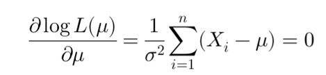
To maximize this log-likelihood, we take the derivative with respect to \(\mu\) and solve the equation:
\[ \frac{d(\log L(\mu))}{d\mu} = \frac{1}{\sigma^2} \sum_{i=1}^{n} (X_i - \mu) = 0 \]
This gives the maximum likelihood estimator for \(\mu\):
\[ \hat{\mu} = \frac{1}{n} \sum_{i=1}^{n} X_i \]
Application to Liquidity Stress Tests
The density of the Generalized Pareto Distribution (GPD) is given by:
\[ f(y; \sigma, \xi) = \frac{1}{\sigma} \left(1 + \xi \frac{y}{\sigma}\right)^{-\frac{1}{\xi} - 1} \]
The log-likelihood is then:
\[ \log L(\xi, \sigma) = -n \log \sigma - \left(1 + \frac{1}{\xi}\right) \sum_{i=1}^{n} \log\left(1 + \xi \frac{y_i}{\sigma}\right) \]
Écrire commentaire